Diffusion Analysis in MD Simulations

Authors: Tyler Reddy and Anna Duncan

The purpose of this Python module is to provide utility functions for analyzing the diffusion of particles in molecular dynamics simulation trajectories using either linear or anomalous diffusion models.

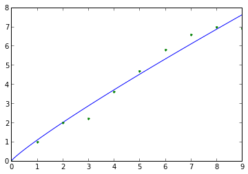
diffusion_analysis.fit_anomalous_diffusion_data(time_data_array, MSD_data_array, degrees_of_freedom=2)

This function should fit anomalous diffusion data to Equation 1 in [Kneller2011], and return appropriate diffusion parameters.

\[MSD = ND_{\alpha}t^{\alpha}\]

An appropriate coefficient (N = 2,4,6 for 1,2,3 degrees_of_freedom) will be assigned based on the specified degrees_of_freedom. The latter value defaults to 2 (i.e., a planar phospholipid bilayer with N = 4). Input data should include arrays of MSD (in Angstroms ** 2) and time values (in ns). The results are returned in a tuple.

Parameters:

time_data_array : array_like

Input array of time window sizes (nanosecond units)

MSD_data_array : array_like

Input array of MSD values (Angstrom ** 2 units; order matched to time_data_array)

degrees_of_freedom : int

The degrees of freedom for the diffusional process (1, 2 or 3; default 2)

Returns:

fractional_diffusion_coefficient

The fractional diffusion coefficient (units of Angstrom ** 2 / ns ** alpha)

standard_deviation_fractional_diffusion_coefficient

The standard deviation of the fractional diffusion coefficent (units of Angstrom ** 2 / ns ** alpha)

alpha

The scaling exponent (no dimensions) of the non-linear fit

standard_deviation_alpha

The standard deviation of the scaling exponent (no dimensions)

sample_fitting_data_X_values_nanoseconds

An array of time window sizes (x values) that may be used to plot the non-linear fit curve

sample_fitting_data_Y_values_Angstroms

An array of MSD values (y values) that may be used to plot the non-linear fit curve

Raises:

ValueError

If the time window and MSD arrays do not have the same shape

References

[Kneller2011]

(1, 2) Kneller et al. (2011) J Chem Phys 135: 141105.

Examples

Calculate fractional diffusion coefficient and alpha from artificial data (would typically obtain empirical data from an MD simulation trajectory):

>>> import diffusion_analysis
>>> import numpy
>>> artificial_time_values = numpy.arange(10)
>>> artificial_MSD_values = numpy.array([0.,1.,2.,2.2,3.6,4.7,5.8,6.6,7.0,6.9])
>>> results_tuple = diffusion_analysis.fit_anomalous_diffusion_data(artificial_time_values,artificial_MSD_values)
>>> D, D_std, alpha, alpha_std = results_tuple[0:4]
>>> print D, D_std, alpha, alpha_std
0.268426206526 0.0429995249239 0.891231967011 0.0832911559401

Plot the non-linear fit data:

>>> import matplotlib
>>> import matplotlib.pyplot as plt
>>> sample_fit_x_values, sample_fit_y_values = results_tuple[4:]
>>> p = plt.plot(sample_fit_x_values,sample_fit_y_values,'-',artificial_time_values,artificial_MSD_values,'.')

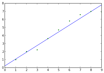
diffusion_analysis.fit_linear_diffusion_data(time_data_array, MSD_data_array, degrees_of_freedom=2)

The linear (i.e., normal, random-walk) MSD vs. time diffusion constant calculation.

The results are returned in a tuple.

Parameters:

time_data_array : array_like

Input array of time window sizes (nanosecond units)

MSD_data_array : array_like

Input array of MSD values (Angstrom ** 2 units; order matched to time_data_array)

degrees_of_freedom : int

The degrees of freedom for the diffusional process (1, 2 or 3; default 2)

Returns:

diffusion_constant

The linear (or normal, random-walk) diffusion coefficient (units of Angstrom ** 2 / ns)

diffusion_constant_error_estimate

The estimated uncertainty in the diffusion constant (units of Angstrom ** 2 / ns), calculated as the difference in the slopes of the two halves of the data. A similar approach is used by GROMACS g_msd [Hess2008].

sample_fitting_data_X_values_nanoseconds

An array of time window sizes (x values) that may be used to plot the linear fit

sample_fitting_data_Y_values_Angstroms

An array of MSD values (y values) that may be used to plot the linear fit

Raises:

ValueError

If the time window and MSD arrays do not have the same shape

References

[Hess2008]

(1, 2) Hess et al. (2008) JCTC 4: 435-447.

Examples

Calculate linear diffusion coefficient from artificial data (would typically obtain empirical data from an MD simulation trajectory):

>>> import diffusion_analysis
>>> import numpy
>>> artificial_time_values = numpy.arange(10)
>>> artificial_MSD_values = numpy.array([0.,1.,2.,2.2,3.6,4.7,5.8,6.6,7.0,6.9])
>>> results_tuple = diffusion_analysis.fit_linear_diffusion_data(artificial_time_values,artificial_MSD_values)
>>> D, D_error = results_tuple[0:2]
>>> print D, D_error
0.210606060606 0.07

Plot the linear fit data:

>>> import matplotlib
>>> import matplotlib.pyplot as plt
>>> sample_fit_x_values, sample_fit_y_values = results_tuple[2:]
>>> p = plt.plot(sample_fit_x_values,sample_fit_y_values,'-',artificial_time_values,artificial_MSD_values,'.')

diffusion_analysis.mean_square_displacement_by_species(coordinate_file_path, trajectory_file_path, window_size_frames_list, dict_particle_selection_strings, contiguous_protein_selection=None, num_protein_copies=None)

Calculate the mean square displacement (MSD) of particles in a molecular dynamics simulation trajectory using the Python MDAnalysis package [Michaud-Agrawal2011].

Parameters:

coordinate_file_path: str

Path to the coordinate file to be used in loading the trajectory.

trajectory_file_path: str or list of str

Path to the trajectory file to be used or ordered list of trajectory file paths.

window_size_frames_list: list

List of window sizes measured in frames. Time values are not used as timesteps and simulation output frequencies can vary.

dict_particle_selection_strings: dict

Dictionary of the MDAnalysis selection strings for each particle set for which MSD values will be calculated separately. Format: {‘particle_identifier’:’MDAnalysis selection string’}. If a given selection contains more than one particle then the centroid of the particles is used, and if more than one MDAnalysis residue object is involved, then the centroid of the selection within each residue is calculated separately.

contiguous_protein_selection: str

When parsing protein diffusion it may be undesirable to split by residue (i.e., amino acid). You may provide an MDAnalysis selection string for this parameter containing a single type of protein (and no other protein types or other molecules / atoms). This selection string may encompass multiple copies of the same protein which should be specified with the parameter num_protein_copies

num_protein_copies: int

The number of protein copies if contiguous_protein_selection is specified. This will allow for the protein coordinates to be split and the individual protein centroids will be used for diffusion analysis.

Returns:

dict_MSD_values: dict

Dictionary of mean square displacement data. Contains three keys: MSD_value_dict (MSD values, in Angstrom ** 2), MSD_std_dict (standard deviation of MSD values), frame_skip_value_list (the frame window sizes)

References

[Michaud-Agrawal2011]

(1, 2) Michaud-Agrawal, E. J. Denning, T. B. Woolf, and O. Beckstein. MDAnalysis: A Toolkit for the Analysis of Molecular Dynamics Simulations. J. Comput. Chem. 32 (2011), 2319–2327

Examples

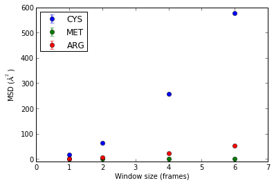
Extract MSD values from an artificial GROMACS xtc file (results measured in A**2 based on frame window sizes) containing only three amino acid residues.

>>> import diffusion_analysis
>>> import numpy
>>> import matplotlib
>>> import matplotlib.pyplot as plt

>>> window_size_list_frames = [1,2,4,6]
>>> dict_particle_selection_strings = {'MET':'resname MET','ARG':'resname ARG','CYS':'resname CYS'}
>>> dict_MSD_values = diffusion_analysis.mean_square_displacement_by_species('./test_data/dummy.gro','./test_data/diffusion_testing.xtc',window_size_list_frames,dict_particle_selection_strings)

Plot the results:

>>> fig = plt.figure()
>>> ax = fig.add_subplot(111)
>>> for residue_name in dict_particle_selection_strings.keys():
...     p = ax.errorbar(window_size_list_frames,dict_MSD_values['MSD_value_dict'][residue_name],yerr=dict_MSD_values['MSD_std_dict'][residue_name],label=residue_name,fmt='o')
>>> a = ax.set_xlabel('Window size (frames)')
>>> a = ax.set_ylabel('MSD ($\AA^2$)')
>>> a = ax.set_ylim(-10,600)
>>> a = ax.legend(loc=2,numpoints=1)